Sleeping Beauties
Kieran Healy posted last year about “sleeping beauties” in philosophy—papers that went several years before receiving any citations but that ended up accumulating many. This pattern is unusual, as most papers receive a good amount of citations immediately and continue to do so (or the opposite). I think literary studies and history is less paper-driven than philosophy, and I would encourage everyone to read this for more context on citations in the humanities.
With that caveat in mind, I decided to check several literary studies journals for any sleeping beauties that I might find. I downloaded the 500 most-cited articles from Critical Inquiry, Representations, PMLA, and New Literary History from Web of Science. The threshold was 20, less than half of the 50 that Healy used for his philosophy corpus. Again, literary scholars just don’t cite journal articles as much as philosophers.
Update 4/8/16: An improved version of the code below can be found here.
You can save the Web of Science “citation report” data as an Excel file and then export it as a csv. You’ll need to delete some graphs and superfluous header information beforehand. After you’ve done so, import it into R:
library(dplyr)
library(tidyr)
library(ggplot2)
sb <- read.csv("citations-sleeping-beauties.csv", stringsAsFactors=FALSE)
This dataframe is a big mess. In order to create a graph similar to Healy’s we’ll need to reshape the data.
sbc <- sb  %>%
   select(Title,Publication.Year,X1973:X2016) %>%
   gather(Year,Each,X1973:X2016) %>%
   mutate(Year = as.numeric(gsub("X","", Year))) %>%
   group_by(Title) %>%
   mutate (Each = cumsum(Each))
This code selects a few columns of interest, switches the wide years to long column format, keeps a cumulative sum, and removes the “X” from the year.
Now we need to keep track of the number of years elapsed since each article was published:
sbcd <- sbc %>% mutate(ELAPSED=Year-Publication.Year) %>% filter (ELAPSED>0)(You can see that I’m keeping copies of each successive data frame around. That’s probably not necessary, but I tend to do it this way for easy revertability.)
For positioning the labels:
sbcd <- sbcd %>% mutate (label_x_position=max(ELAPSED))
sbcd <- sbcd %>% mutate(label_position=max(Each))
Plotting the graph could be done with:
gg <- ggplot(data=sbcd, aes(x=ELAPSED,y=Each, Group=Title))
    gg <- gg + theme_bw()
    gg <- gg + geom_line(colour="gray", alpha=.25)
    gg <- gg + scale_y_continuous(trans=log2_trans())
    gg <-  gg + xlab("Years Elapsed Since Publication")
    gg <-  gg + ylab("Cumulative Citations")
    gg <-  gg + ggtitle("Sleeping Beauties in Literary Studies")
    gg <- gg + geom_text(data=subset(sbcd, Each <1 & ELAPSED > 10), aes(x=label_x_position, y=label_position, Group=Title, label=Title), colour="red", size=2)
   gg
To highlight the articles that are the sleeping beauties in the plot itself, I first had to create a separate dataframe:
rt <- sbcd %>% filter(grepl("STOKER|SENSATION|16TH-CENTURY SPAIN",Title))And then add another layer:
gg <- gg + geom_line(data=rt, aes(x=ELAPSED, y=Each, Group=Title), alpha=1, colour="red")This process is not obviously not ideal, as it relies on a manual matching regular expression and requires trial-and-error. Just getting to this point was a major pain, however, and I still haven’t matched Healy’s y-scale.
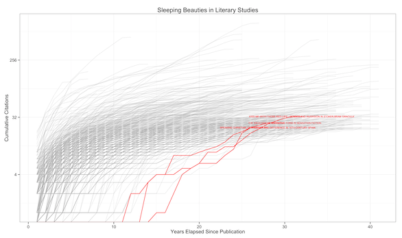
In any case, the resulting graph will look like:
The three articles are Christopher Craft’s "‘Kiss Me with those Red Lips’: Gender and Inversion in Bram Stoker’s Dracula," Jonathan Loesberg’s “The Ideology of Narrative Form in Sensation Fiction,” and Deborah Root’s “Speaking Christian: Orthodoxy and Difference in Sixteenth-Century Spain.” All three are from Representations, and all were published in the 1980s. I could speculate about why these papers went more than ten years without gathering any citations in the Web of Science database, but I’d first want to check to see if that’s not an artifact in the data. There were clearly citations that WoS missed for the Craft article, as google scholar reveals. The Loesberg and Root articles are closer to true “sleeping beauties,” but there were missed citations with them as well.
As with most literary studies citation analyses based on journal data, the results are incomplete, confusing, and disappointing. I hold out hope that book data will be readily available one day.
UPDATE
I’ve created a d3.js voronoi tessellated line chart of some of this data. It doesn’t have a log scale, and it’s filtered so that only articles with more than 50 citations appear. The code is taken from Mike Bostock, this Stackoverflow answer, and in particular this example from Lynn Cherny.
